Kurtosis
In probability theory and statistics, kurtosis (from the Greek word κυρτός, kyrtos or kurtos, meaning bulging) is any measure of the "peakedness" of the probability distribution of a real-valued random variable.[1] In a similar way to the concept of skewness, kurtosis is a descriptor of the shape of a probability distribution and, just as for skewness, there are different ways of quantifying it for a theoretical distribution and corresponding ways of estimating it from a sample from a population.
One common measure of kurtosis, originating with Pearson, is based on a scaled version of the fourth moment of the data or population, but it has been argued that this measure really measures heavy tails, and not peakedness.[2] For this measure, higher kurtosis means more of the variance is the result of infrequent extreme deviations, as opposed to frequent modestly sized deviations. An alternative measure, the L-kurtosis is a scaled version of of the fourth L-moment.
Contents |
Pearson moments
The fourth standardized moment is defined as

where μ4 is the fourth moment about the mean and σ is the standard deviation. This is sometimes used as the definition of kurtosis in older works, but is not the definition used here.
Kurtosis is more commonly defined as the fourth cumulant divided by the square of the second cumulant, which is equal to the fourth moment around the mean divided by the square of the variance of the probability distribution minus 3,
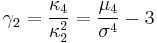
which is also known as excess kurtosis. The "minus 3" at the end of this formula is often explained as a correction to make the kurtosis of the normal distribution equal to zero. Another reason can be seen by looking at the formula for the kurtosis of the sum of random variables. Suppose that Y is the sum of n identically distributed independent random variables all with the same distribution as X. Then
![\operatorname{Kurt}[Y] = \frac{1}{n}\operatorname{Kurt}[X]](/2012-wikipedia_en_all_nopic_01_2012/I/9d8b393003c78024cfd38ba7818d9286.png)
This formula would be much more complicated if kurtosis were defined just as μ4 / σ4 (without the minus 3).
More generally, if X1, ..., Xn are independent random variables, not necessarily identically distributed, but all having the same variance, then
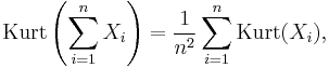
whereas this identity would not hold if the definition did not include the subtraction of 3.
The fourth standardized moment must be at least 1, so the excess kurtosis must be −2 or more. This lower bound is realized by the Bernoulli distribution with p = ½, or "coin toss". There is no upper limit to the excess kurtosis and it may be infinite.
Terminology and examples
A high kurtosis distribution has a sharper peak and longer, fatter tails, while a low kurtosis distribution has a more rounded peak and shorter, thinner tails.
Distributions with zero excess kurtosis are called mesokurtic, or mesokurtotic. The most prominent example of a mesokurtic distribution is the normal distribution family, regardless of the values of its parameters. A few other well-known distributions can be mesokurtic, depending on parameter values: for example the binomial distribution is mesokurtic for  .
.
A distribution with positive excess kurtosis is called leptokurtic, or leptokurtotic. "Lepto-" means "slender"[1]. In terms of shape, a leptokurtic distribution has a more acute peak around the mean and fatter tails. Examples of leptokurtic distributions include the Cauchy distribution, Student's t-distribution, Rayleigh distribution, Laplace distribution, exponential distribution, Poisson distribution and the logistic distribution. Such distributions are sometimes termed super Gaussian.
A distribution with negative excess kurtosis is called platykurtic, or platykurtotic. "Platy-" means "broad"[2]. In terms of shape, a platykurtic distribution has a lower, wider peak around the mean and thinner tails. Examples of platykurtic distributions include the continuous or discrete uniform distributions, and the raised cosine distribution. The most platykurtic distribution of all is the Bernoulli distribution with p = ½ (for example the number of times one obtains "heads" when flipping a coin once, a coin toss), for which the excess kurtosis is −2. Such distributions are sometimes termed sub Gaussian.
Graphical examples
The Pearson type VII family
The effects of kurtosis are illustrated using a parametric family of distributions whose kurtosis can be adjusted while their lower-order moments and cumulants remain constant. Consider the Pearson type VII family, which is a special case of the Pearson type IV family restricted to symmetric densities. The probability density function is given by
![f(x; a, m) = \frac{\Gamma(m)}{a\,\sqrt{\pi}\,\Gamma(m-1/2)} \left[1%2B\left(\frac{x}{a}\right)^2 \right]^{-m}, \!](/2012-wikipedia_en_all_nopic_01_2012/I/794af7dc4ff6be340212744f6a2e4a01.png)
where a is a scale parameter and m is a shape parameter.
All densities in this family are symmetric. The kth moment exists provided m > (k + 1)/2. For the kurtosis to exist, we require m > 5/2. Then the mean and skewness exist and are both identically zero. Setting a2 = 2m − 3 makes the variance equal to unity. Then the only free parameter is m, which controls the fourth moment (and cumulant) and hence the kurtosis. One can reparameterize with  , where
  is the kurtosis as defined above. This yields a one-parameter leptokurtic family with zero mean, unit variance, zero skewness, and arbitrary positive kurtosis. The reparameterized density is

In the limit as  one obtains the density
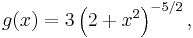
which is shown as the red curve in the images on the right.
In the other direction as  one obtains the standard normal density as the limiting distribution, shown as the black curve.
In the images on the right, the blue curve represents the density  with kurtosis of 2. The top image shows that leptokurtic densities in this family have a higher peak than the mesokurtic normal density. The comparatively fatter tails of the leptokurtic densities are illustrated in the second image, which plots the natural logarithm of the Pearson type VII densities: the black curve is the logarithm of the standard normal density, which is a parabola. One can see that the normal density allocates little probability mass to the regions far from the mean ("has thin tails"), compared with the blue curve of the leptokurtic Pearson type VII density with kurtosis of 2. Between the blue curve and the black are other Pearson type VII densities with γ2 = 1, 1/2, 1/4, 1/8, and 1/16. The red curve again shows the upper limit of the Pearson type VII family, with
  (which, strictly speaking, means that the fourth moment does not exist). The red curve decreases the slowest as one moves outward from the origin ("has fat tails").
Kurtosis of well-known distributions
In this example we compare several well-known distributions from different parametric families. All densities considered here are unimodal and symmetric. Each has a mean and skewness of zero. Parameters were chosen to result in a variance of unity in each case. The images on the right show curves for the following seven densities, on a linear scale and logarithmic scale:
- D: Laplace distribution, a.k.a. double exponential distribution, red curve (two straight lines in the log-scale plot), excess kurtosis = 3
- S: hyperbolic secant distribution, orange curve, excess kurtosis = 2
- L: logistic distribution, green curve, excess kurtosis = 1.2
- N: normal distribution, black curve (inverted parabola in the log-scale plot), excess kurtosis = 0
- C: raised cosine distribution, cyan curve, excess kurtosis = −0.593762...
- W: Wigner semicircle distribution, blue curve, excess kurtosis = −1
- U: uniform distribution, magenta curve (shown for clarity as a rectangle in both images), excess kurtosis = −1.2.
Note that in these cases the platykurtic densities have bounded support, whereas the densities with positive or zero excess kurtosis are supported on the whole real line.
There exist platykurtic densities with infinite support,
- e.g., exponential power distributions with sufficiently large shape parameter b
and there exist leptokurtic densities with finite support.
- e.g., a distribution that is uniform between −3 and −0.3, between −0.3 and 0.3, and between 0.3 and 3, with the same density in the (−3, −0.3) and (0.3, 3) intervals, but with 20 times more density in the (−0.3, 0.3) interval
Sample kurtosis
For a sample of n values the sample kurtosis is
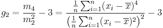
where m4 is the fourth sample moment about the mean, m2 is the second sample moment about the mean (that is, the sample variance), xi is the ith value, and  is the sample mean.
Estimators of population kurtosis
Given a sub-set of samples from a population, the sample kurtosis above is a biased estimator of the population kurtosis. The usual estimator of the population kurtosis (used in DAP/SAS, Minitab, PSPP/SPSS, and Excel but not by BMDP) is G2, defined as follows:
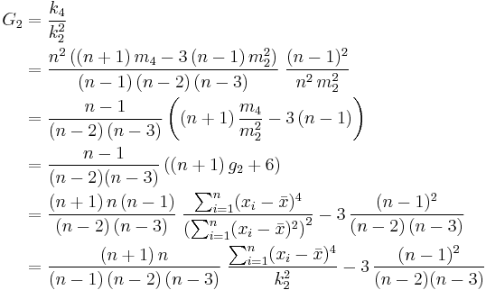
where k4 is the unique symmetric unbiased estimator of the fourth cumulant, k2 is the unbiased estimator of the population variance, m4 is the fourth sample moment about the mean, m2 is the sample variance, xi is the ith value, and  is the sample mean. Unfortunately,
  is itself generally biased. For the normal distribution it is unbiased.
Applications
D'Agostino's K-squared test is a goodness-of-fit normality test based on a combination of the sample skewness and sample kurtosis, as is the Jarque-Bera test for normality.
Other measures of kurtosis
A different measure of "kurtosis", that is of the "peakedness" of a distribution, is provided by using L-moments instead of the ordinary moments.[3][4]
See also
References
- ^ Dodge, Y. (2003) The Oxford Dictionary of Statistical Terms, OUP. ISBN 0-19-920613-9
- ^ SAS Elementary Statistics Procedures, SAS Institute (section on Kurtosis)
- ^ Hosking, J.R.M. (1992). "Moments or L moments? An example comparing two measures of distributional shape". The American Statistician 46 (3): 186–189. JSTOR 2685210.
- ^ Hosking, J.R.M. (2006). "On the characterization of distributions by their L-moments". Journal of Statistical Planning and Inference 136: 193–198.
Further reading
- Joanes, D. N. & Gill, C. A. (1998) Comparing measures of sample skewness and kurtosis. Journal of the Royal Statistical Society (Series D): The Statistician 47 (1), 183–189. doi:10.1111/1467-9884.00122
- Kim, Tae-Hwan; & White, Halbert. (2003/4). "On More Robust Estimation of Skewness and Kurtosis: Simulation and Application to the S&P500 Index". Finance Research Letters, 1, 56-70 doi:10.1016/S1544-6123(03)00003-5 Alternative source (Comparison of kurtosis estimators)
- Seier, E. & Bonett, D.G. (2003). Two families of kurtosis measures. Metrika, 58, 59-70.
External links
- Free Online Software (Calculator) computes various types of skewness and kurtosis statistics for any dataset (includes small and large sample tests)..
- Kurtosis on the Earliest known uses of some of the words of mathematics
- Celebrating 100 years of Kurtosis a history of the topic, with different measures of kurtosis.
|
|||||||||||||||||||||||||||||||||||||||||||||||||||||||||||||||||||||||||||||||||||||||||||||||||||||||||||||||||||||||||||||||||||||||||||